Probe Monitors — A Detector, and Honest Evidence About It

A probe monitor is a small linear readout over one decoder layer's residual stream: a vector and a threshold that answer is this concept present in what the model is processing right now? Nothing about it is exotic — it is logistic regression on activations. What the panel is really for is the second half: finding out how well it actually works, and not overstating it.

A probe is cheap to run next to a model, which is the whole appeal. A 7B judge reading the same text costs a forward pass per check; a probe costs a dot product. That trade is only worth making if you know what you are giving up, so this feature spends most of its effort on measurement.

---

What a probe is, exactly

It helps to be concrete, because the word "probe" invites a mental model that fits only half of what miStudio builds.

The dense probe: one vector, no latents

A dense probe — the default, and what the tile labels dense residual — is literally this:

weight   d_model numbers   (2,048 for LFM2.5-1.2B, 4,096 for Llama-3.1-8B)
bias     1 number

score(token) = standardise(activation at layer L) · weight + bias

That is the entire artifact. There are no feature detectors inside it, nothing that "activates", and no dictionary. It is one dot product against the residual stream, which is why it costs almost nothing to run beside a model: the forward pass was happening anyway, and the probe adds a vector multiply at one layer.

The k-sparse SAE probe: one weight per latent

A probe can instead read an SAE's feature basis. Training encodes the activations through the SAE, ranks the features by a standardised class-mean difference on the training rows only, keeps the top k, and learns one weight per kept feature.

This is the version where "latents activate and the probe reads them" is an accurate description. The tile shows it as an SAE basis with its feature count instead of dense residual.

	dense	k-sparse SAE
what it reads	the raw residual stream	the SAE's feature activations
size	d_model weights	k weights
needs an SAE?	no	yes, and a published one to export
interpretable per-weight?	not really	yes — each weight names a feature

It is never told which tokens matter

Worth knowing before you read a token trace: training minimises binary cross-entropy on the pooled aggregate against the whole-input label. Nothing supervises individual tokens. The per-token scores the trace shows are a by-product you can inspect, not a target the probe was fitted to. That is why a single strongly-coloured token does not mean "the probe fired here".

---

The evidence ladder

Every probe carries a rung, and the rung is computed from the evidence, never asserted:

rung	what it means
0	trained — a probe exists and fit its training data
1	detects on held-out data — it works on rows it did not see, from the same distribution
2	detects on unseen tasks — it works on every out-of-distribution evaluation set run (the lower bound of a bootstrapped confidence interval clears chance on each), and at its shipped bar it catches at least half the positives on each of them, and it stays quiet on everyday text and on nonsense text (What rung 2 requires)
3	detects on unseen tasks, compared with a judge — an LLM judge scored the same rows, so the probe's number has something to be read against

What rung 2 requires

Rung 2 (detects on unseen tasks) is reached only when all four of these hold. Each is computed from evaluations that exist; a condition nobody has measured counts as not met.

#	condition	measured on	setting (Settings → Environment)
1	Ranking on unseen tasks — the lower bound of the AUROC confidence interval is above 0.5	every out-of-distribution evaluation set (at least one)	—
2	Catch rate — at the shipped bar (score ≥ the probe's threshold), it catches at least 50% of the positives	each of those same out-of-distribution sets	Rung 2 catch rate, rung2_min_recall (0.5)
3	Everyday text — false alarms at the shipped bar at most 2× the target rate, on a set of at least 1,000 rows	an everyday_text view (ordinary prose)	everyday_text_fpr_factor (2), everyday_text_min_rows (1,000)
4	Nonsense text — false alarms at the shipped bar at most 2× the target rate, on a set of at least 1,000 rows	a nonsense_text view (word salad, random characters, repeated tokens, garbled code…)	nonsense_text_fpr_factor (2), nonsense_text_min_rows (1,000)

When any of 2–4 fails, the probe is held at rung 1 (rung 0 without an in-distribution pass), every failing condition is named in its reasons, and its next step is the first of them, in the order above. The report shows each in plain words:

• On unseen tasks (carriers): catches 10% of positives at the shipped bar (41 of 410; needs ≥ 50%) — and the reason catches 10% of positives on unseen tasks at the shipped bar (needs ≥ 50%);
• On everyday text: 0 false alarms in 1,200 (allowed up to 24), Fired on 100% of everyday text, or not yet checked on everyday text — evaluate on an everyday-text set;
• On nonsense text: 41 false alarms in 2,000 (allowed up to 40), or not yet checked on nonsense text — evaluate on a nonsense-text set.

Why the catch rate (2). Conditions 1, 3 and 4 can all be met by a probe that almost never fires. On one personal-data run, three max probes passed the everyday-text check with 0% false alarms because they fire on almost nothing — at their shipped bar they caught at most 2.5% of the positives they were for. The run's own pick ranked unseen tasks best (AUROC 0.787) and caught 10% at its bar. Ranking is what AUROC measures; a monitor is judged at one bar, so rung 2 now asks what happens there. It is measured at the shipped bar, never at a bar cut on the evaluation set itself — that one is tuned to the set and says nothing about the deployed probe. The positives' scores are kept, so after a re-cut the catch rate is taken again at the new bar.

Why nonsense text (4). Prose and gibberish are different failure surfaces. The layer-0 mean probe of that run passed the everyday-text check (0.35%) and fired on all 280 benchmark chats made of random common words strung together.

Getting a nonsense-text set. No GPU and no download: ask the agent to run create_nonsense_text_dataset (MCP), or POST /api/v1/probe-monitors/nonsense-text ({"rows": 2000, "seed": 0}). It writes a seeded dataset — the same seed gives the same rows — with columns text and kind, mixing word salad from common words, random characters, one token repeated, garbled code, digit noise, mixed scripts and, given prose_dataset_id (a downloaded prose corpus such as an OpenWebText sample), shuffled sentences of real prose; lengths run from a token to about 4,000. Without a prose corpus that kind is skipped, and the response's manifest.skipped says so. No row is ever SSN-shaped: digit noise is built from groups of at most 8 digits with separators of at least 4 characters, and a final pass over every row breaks any run of 9 digits and any 3-2-4 digit grouping. The same call registers the nonsense_text view (every row a negative, grouped by kind, so a breakdown shows which kind fires); then evaluate the probe on it.

Probes rated before 2026-10-29's second change (ENH-006 D84) were re-stated to rung 1 (or 0) with the reason not yet checked on nonsense text, and their local definitions marked invalidated: no nonsense-text set could exist before. Published exports are not changed.

Rung 2 also needs everyday text

Since 2026-10-29 a probe reaches rung 2 only when it has also been evaluated on an everyday-text set — ordinary writing with nothing of any behaviour in it — and fires rarely there at the bar it ships with. Precisely:

• at least one evaluation on a view whose role is everyday text (everyday_text), with at least 1,000 rows (the deployment setting Everyday-text set size, everyday_text_min_rows);
• on every such set of that size, the share of rows scoring at or above the shipped threshold is at most twice the probe's target false-positive rate (Everyday-text allowance, everyday_text_fpr_factor): with a 1% target, at most 2% — 24 rows of 1,200.

Otherwise the probe is held at rung 1 (rung 0 if no in-distribution set passed), and its reasons and next step say which: not yet checked on everyday text — evaluate on an everyday-text set, or false alarms on everyday text 100% at the shipped bar (allowed ≤ 2%). The report shows each set in plain words — On everyday text: 0 false alarms in 1,200 (allowed up to 24), or Fired on 100% of everyday text. A smaller set is shown but does not count.

Why. An out-of-distribution set for a behaviour is still a set about that behaviour, so it never asked whether a probe fires on plain prose. When random everyday words were sent through a served model with the nine probes of one personal-data run armed, the right answer was "absent" every time — and one layer-0 probe fired on all 280 inputs, another on half of them, while both were rated rung 2. A probe like that would flood a monitor with false alarms on real traffic.

The count follows the bar. The rows' scores are kept, so when the threshold is re-cut the false-alarm count is taken again at the new bar and the rung recomputed. Probes rated before this rule were re-stated to rung 1 (or 0) with the reason not yet checked on everyday text, and any definition built for them locally was marked invalidated. Exports already published — to the Hub or into miLLM — are not changed: an export records its rung as of the day it was built.

Getting an everyday-text set. One set serves every probe and every model:

1. Download a corpus of ordinary writing on the Datasets screen — for example an OpenWebText sample (web pages) or a general-chat corpus already on this installation. Text is all it needs.
2. On Probes → Datasets, create a view over it with Role: everyday text. Pick the text column as the input and any column — the text column itself will do — as the label column: every row is read as a negative (through the API or MCP, send label_mapping: {"*": "negative"}; that wildcard is accepted on this role only). A view of this role refuses a positive mapping, a behaviour, a sub-question and a distribution.
3. Evaluate the probe on it (Evaluate on more sets on its report, or evaluate_probe_monitor). A large corpus can be evaluated on a seeded sample (sample_rows, for example 2,000): the same rows for every probe evaluated at that size.

Two things about rung 3 are deliberate and easy to misread.

"Compared with", not "beats". A probe at rung 3 has been measured against a judge. It may have lost. On the reference run it did lose — the judge averaged 0.8744 across five sets against the probe's 0.7938, and won on all five individually. That is recorded rather than buried, because a rung-3 badge could otherwise be read as "better than asking a model", which it does not mean. The probe's case on a small model is cost and latency, not accuracy.

Only a judge of the same behaviour counts. Since 2026-10-21 rung 3 is reached only by a judge run whose judge prompt judges the same behaviour as the probe — the probe's behaviour key (set when the run is started, or later on the probe's report) must equal the prompt's. A judge of another behaviour (a high-stakes rater compared with a personal-data probe) still runs and is still shown, but it never raises the rung, and the report says why. The judge must also have scored the set: a set it could not score (too few readable replies) does not count. The rung's reasons state the judge's prompt, model and how many rows per set it read.

The rung moves, and a stale export is invalidated. Run another evaluation or a judge pass and the rung is recomputed. If it changes, any definition already built is marked invalidated rather than silently left in place — a cached document stating an old rung is a lie that still parses.

---

Running one, field by field

The panel is Probes in the sidebar, between Circuits and J-Lens. Everything needed to start a run is on that one page, above the list of past runs. Filling it in, top to bottom:

control	what to put in it
Model	The model whose residual stream you are reading. It must already be downloaded (Models panel).
Training view	The labelled dataset the probe learns from. This is a view, not a raw dataset — see below.
Evaluation sets	Tick any number. Each is marked OOD (out-of-distribution) or in-distribution, and that marking is what decides whether a run can reach rung 2.
Calibration set	Leave as "none — use validation negatives" unless you have a set of known-negatives you would rather calibrate the threshold on.
Scope	all, assistant, user or last_assistant. The panel says it plainly: these are different detectors, not a preference.
GPU	Auto — most free memory is right almost always.
Layers	stride walks the stack (stride 5 over 16 layers gives layers 1, 6, 11); explicit takes a list like 11,12,13. The run trains a probe at each and keeps the best.
Rules	The pooling rules to try: mean, max, last, softmax, attention, rolling_mean_max. Tick several — the run picks the winner by validation AUROC and shows you the whole sweep.
Max length	Token cap per row. 4096 is the default.
Top-N layers	How many layers to carry forward from the sweep. 1 is normal.
Target FPR	The false-positive rate the threshold is calibrated to. 0.01 is the default.
Seed	1337 by default. The same seed gives the same split, the same capture order and the same initialisation — which is what makes two runs comparable.
SAE variant	Also trains a k-sparse probe over an SAE basis. It needs a ready residual SAE for that model at the selected layer, or the run is refused naming the layer.

Then Start probe run.

If "Training view" is empty, that is the step you are missing

A probe cannot read a raw dataset. It needs a view: which column holds the text, which column holds the label, and what each raw label value means — positive, negative or excluded. A view that cannot produce both classes is refused when you create it, rather than forty minutes into a run.

Views are created against a dataset you have already downloaded, and each one is tagged with a role (train, eval, calibration, or everyday_text — ordinary prose with no positives, which rung 2 checks false alarms on) and, for evaluation views, a distribution (in-distribution or OOD). The existing views on this installation are named like models-under-pressure training (train) and models-under-pressure mt_balanced — one training view and five OOD evaluation sets over the same source dataset.

Registering a view with a miDataworks manifest

A view can be registered with the dataset-version manifest miDataworks publishes beside each dataset version (dataset_version_manifest on POST /api/v1/probe-monitors/datasets; miDataworks sends it itself when it hands a detector set over). Over MCP, register_probe_dataset takes dataset_version_id instead and fetches the manifest from miDataworks, so the document need not pass through the call; with miDataworks absent it answers {"unavailable": "dataworks", …} and registers nothing, never an unverified view. It is optional — without one, registration is exactly as above. With one, miStudio checks it before it keeps the view:

Refusal	When
422, naming the failing JSON path (e.g. $.version.number)	The manifest is not valid against miDataworks' schema (midataworks-dataset-version-v1.json, vendored byte-identical)
422 "name the split"	A manifest is sent without split — a manifest describes splits by name, so the check needs one
409, listing the manifest's splits	The split being registered is not described by the manifest
409, naming both counts	The manifest's row count for the split differs from the downloaded split's. The comparison is made before the keyword filter and label mapping, which are miStudio's own narrowing

What was verified is recorded on the view as dataset_version — version id and number, dataset name, split, both row counts, repository, commit and the manifest's SHA-256 — and returned by the create and list calls. A version that is not published yet has no commit, and the record says null rather than guessing one. The commit is the manifest's claim: miStudio's download does not pin a revision, so it is recorded, not re-verified.

Browsing a dataset's rows

On the Datasets tab, click a dataset's name (or Rows) to open its rows. Nothing here can be edited. Each row shows:

• its input text (a conversation is shown as role: text lines), cut at 160 characters with more to expand it;
• its label as the view reads it — Positive, Negative, Excluded, Filtered out (dropped by the view's keyword filter) or Unreadable (an input that could not be read as text or a conversation, or a raw label the mapping does not name) — with the raw value under it;
• the pair column, if the view has one, and the dataset's other columns. Untick a column under Other columns to hide it.

The counts at the top are the ones recorded when the view was created, and the labels in the table come from the same rule that produced them, so clicking a count shows exactly that many rows. Search the input text narrows to rows whose input contains the text (case doesn't matter), and Rows per page sets the page size (25 to 200). A label filter re-reads the whole dataset once; if the downloaded data has changed since the view was made, an amber note says so and gives the new counts — runs on the view were submitted against the recorded ones.

Agents read the same rows with the MCP tool get_probe_dataset_rows (paged, with columns to fetch only the columns they need).

Archiving and deleting datasets

Two steps, the same as in miDataworks and miForge:

• Archive hides a dataset from this tab and from the run, evaluation and judge forms. Nothing is deleted: every run, probe and evaluation that already uses it keeps working, and Unarchive (with Show archived ticked) brings it back. A new run that names an archived dataset is refused (409). Agents can archive and unarchive (archive_probe_dataset, unarchive_probe_dataset); the tab shows who archived a dataset, when (ET) and why.
• Delete permanently removes an archived dataset's definition — its columns, label mapping and counts — for good. Tick Show archived: each archived dataset gets a checkbox, the header has Select all / Deselect all (half-ticked when only some are selected) and a live "N selected" count, and Delete permanently opens a confirmation listing what goes and what is skipped, with an optional reason that is kept in the record. Delete… on any row does the same in one step: it archives the dataset and then deletes it, after the same confirmation.

A dataset cannot be deleted while anything still uses it. The row says why, and its checkbox is greyed out:

Shown as	What it means	What to do
a run is running / pending	a probe run uses it for training, evaluation or calibration and has not finished	wait, or stop the run
a run uses it	a finished run still exists that used it (deleting the dataset would delete that run and its probes, or erase where their threshold came from)	delete the run on the Runs tab first, if it should go too
a probe's threshold / an evaluation	a probe was calibrated or evaluated on it outside its run	keep the dataset; this is evidence
a judge baseline	an LLM-judge baseline was measured on it	keep it, or delete that baseline's probe run
an agent request	an agent's request that names it is waiting for your approval, or approved and not yet used	deny it, or let it run

The downloaded data is not deleted. A probe dataset is a view over a download, not a copy, and the download may be read by other probe datasets, tokenizations and extractions; delete it from the Datasets screen if you want it gone. Each permanent delete leaves a record — who, when, why and the dataset's full definition — that cannot be edited or removed (GET /api/v1/probe-monitors/dataset-purges). Deleting is the operator's alone: there is no MCP tool for it, and the server refuses a delete that comes through the MCP server. Like Delete on the Runs tab, it asks for confirmation rather than the Settings PIN.

What a good first run looks like

Nothing exotic: one model, the training view, all the evaluation sets, scope all, stride layers, and two or three rules. That gives you a layer sweep to look at and a probe at the end. A run with no evaluation sets is also allowed and gives you a rung-0 probe — worth doing if all you want to know is whether a concept is linearly present at all.

Three settings that change the answer, not just the speed

Most of the form is bookkeeping. These three are not.

• Pooling rule. How per-token scores become one score for a row. On the reference corpus mean reached 0.8841 out of distribution while attention reached 0.6986 — and the attention probe was not under-trained: it converged to a lower training loss and generalised far worse. Tick several and let the run choose.
• Scope. Which tokens may be scored. Template scaffolding is never scored under any scope, because including a BOS token would make a mean rule's denominator depend on the chat template rather than on the text.
• Layers. The run keeps the best by validation AUROC, and the tile says when that choice was close: "margin over the runner-up 0.0012 — a near-tie, so the chosen layer is close to arbitrary." Treat a near-tie as "any of these layers", not as a finding about layer 11.

---

What a run actually does

One run is not one probe. A run sweeps, trains, calibrates and evaluates, and hands back several probes for you to choose between. Its eight stages appear on the tile as it works, and a failure names the stage it failed at.

stage	what happens
rendering	each labelled row becomes the token ids the model will really see, with the chat template applied
pooled_capture	the model runs over the training rows; one pooled activation is kept per row, per candidate layer
layer_selection	the sweep — a cheap probe is fitted at every layer × pooling rule and scored on validation
token_capture	the chosen layer is re-run, this time keeping per-token activations
training	AdamW and BCE on the aggregate, early stopping on validation AUROC
calibrating	the threshold is placed at the score that spends your target false-positive rate on validation negatives
evaluating	the held-out sets are scored: AUROC, bootstrap CI, operating points
rung	the evidence rung is derived from what actually ran

Two details in there are easy to miss and change how you read the output.

Early stopping watches AUROC, not loss. They do not share a minimum. Stopping on loss can hand back a probe that separates the classes worse than one seen several epochs earlier.

The threshold is calibrated on validation negatives, and it rarely lands on your target. Asking for 1% typically yields something like 0.97% or 0.82%, because scores are discrete at the sample level. The tile shows what was actually spent, not what you asked for — those are different numbers and only one of them is true.

Why one run produces four tiles

mean, max, last and attention are four pooling rules over the same readout. The run scores all four and selects a winner on validation AUROC, but keeps them all, because the winner in-distribution is not always the winner out of it. On the reference run, attention reached a lower training loss than mean and generalised distinctly worse — which is what overfitting looks like when you have the evidence to see it.

---

Reading the run tiles

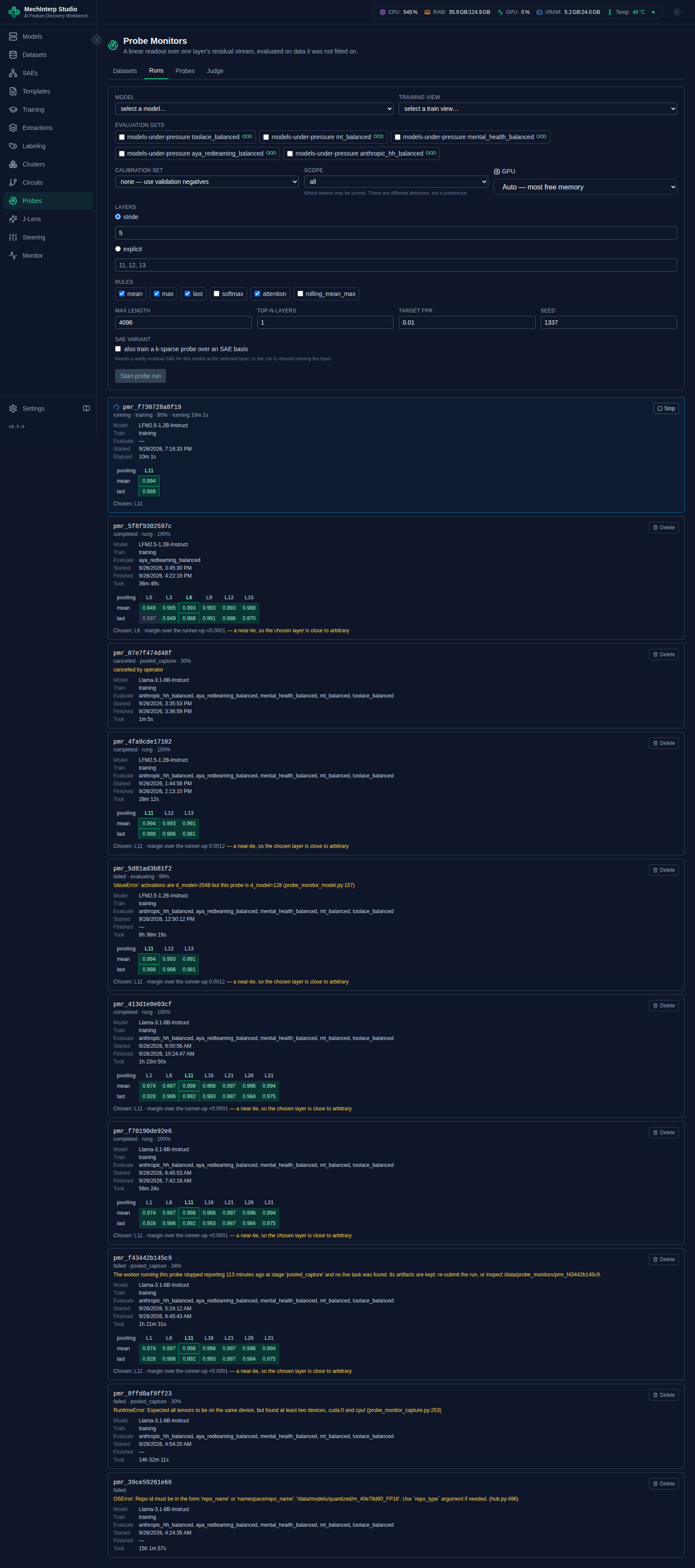
One tile per run, newest first. Each carries:

• the run id, its status, the stage it is in and a percentage — the stage matters, because "40%" means nothing without pooled_capture or evaluating beside it;
• a spinner and a progress bar while it is live, the same bar every other running job in miStudio draws, and under it what the bar is counting: the step (for example Capturing token activations, step 4 of 8), how many of its units are done (120 of 400 batches, 2 of 8 probes, 1 of 3 sets), the item inside the step (a probe's epochs, an evaluation set's batches), the speed and the time left in that step — marked (provisional, still measuring) until the step has run 25 batches and two minutes, because the first batches of a set can read thirty hours that become ninety minutes once the speed settles. The tile refreshes every 5 seconds and the run writes a new reading every 10, so a step that is slow but moving no longer looks stuck;
• the datasets it is actually using — model, training view, and every evaluation set by name rather than by id;
• when it started, when it finished, and how long it took;
• the layer sweep it chose from, as a small table of rule against layer, and which layer won.

A run that failed shows its error on the tile. A run whose end was never recorded shows Took — rather than a duration counted up to the present moment: a made-up number is worse than a blank, because you cannot tell it is made up.

Stop appears while a run is live and Delete once it is not. Stopping is cooperative — work halts at the next clean boundary rather than being killed, so the GPU is released properly and the row does not end up in a state nothing can read. Deleting removes the run, every probe trained in it, and its artifact directory, which is gigabytes of token capture; the tile asks first and says so.

---

Try it on your own text, and read the trace

Try it on your own text scores one input and shows what every token contributed. It is the fastest way to find out whether a probe reads the concept or reads something correlated with it.

The two colours

	meaning
violet	this token pushed the score up — toward the concept
emerald	this token pushed the score down — away from it
<|…|> chip	chat-template scaffolding, not your words
dotted underline	outside this probe's scope, so not scored at all

That last row matters more than it looks. A token outside the scope has no score — it is not a zero. Shading it as "cold" would say the probe looked and found nothing, when it never looked.

Scaffolding is marked rather than hidden, deliberately. A probe firing on <|im_start|> rather than on your sentence is a finding, and filtering those tokens out would delete the evidence for it. With scope all, a chat-rendered input genuinely does score its template tokens.

The four bands, and what they are not

Shading is banded — faint, weak, moderate, strong — and each band moves three things together: background strength, text colour, and an underline rule. One channel alone is not legible across a long passage.

⚠ The bands rank tokens against each other within one input. They are cut against the 90th percentile of the magnitudes in that input, not against any fixed scale. Two consequences:

• Bands do not compare between two inputs. A "strong" token in a passage that scored far below threshold is still part of a low score.
• Two tokens in the same band are not ranked against each other. Hover for the exact number.

The percentile is there because the alternative does not work. Scores are heavy-tailed: on a real 90-token input the largest magnitude was 33.24 while the median was 4.23, so cutting bands against the maximum put 86 of those 90 tokens into the bottom two bands and the whole passage rendered as one flat wash.

Only the aggregate decides

The per-token scores are pooled by the probe's rule into a single aggregate, and the aggregate alone is compared with the threshold. A strongly-coloured token does not mean the probe fired, and a probe that fired does not mean any particular token caused it. The trace tells you where the signal was distributed; the aggregate tells you what the probe concluded.

---

Exporting a probe

A trained probe is only useful if something else can run it. Export writes a mistudio.probe-definition/v1 document: the layer and hook point, the weight vector and bias, the pooling rule, the operating point, the model pinned to a commit (never a branch — the same repository at another revision is a different distribution), the evidence with its rung, and a set of verification vectors.

What export refuses, and why

• Below rung 2 — refused unless you send an acknowledgement recording who accepts that and why. The acknowledgement then travels inside the document, at evidence.acknowledgement, so whoever receives the file cannot miss that its evidence was waived.
• A probe with no evaluations at all — refused even with an acknowledgement, because the document would carry no parity check. An acknowledgement waives evidence about the concept; it cannot manufacture a way to verify the file.
• A k-sparse probe whose SAE has no HuggingFace location — refused, and not waivable. A consumer cannot encode into the SAE basis without the dictionary, so the SAE has to be published first.
• A model with no repository id — refused rather than falling back to its display name, which is a string nobody can fetch in the one field that says what to fetch.

⚠ Score token_ids, not messages

The verification vectors exist so a consumer can confirm it implemented the probe correctly. Each one carries messages, token_ids, per-token scores and a final score — and the token_ids are authoritative.

This is not a style preference, it is measured per export. On a corpus of plain prose — not conversations — the exporter has to reconstruct something sendable, so it wraps each row as a single user turn. Re-rendering that through the model's chat template adds tokens the scored row never had. Measured on the reference definition, sixteen vectors:

scored from	maximum difference from the recorded score
the recorded token_ids	0.000 — exact, all sixteen
messages, re-rendered	1.153 — 23× the suggested tolerance

Every definition states test_vectors.authoritative_input and carries messages_reproduce_token_ids, which the exporter measures by re-rendering its own messages and comparing. The export panel warns when that check came back false, because the person exporting is the last one who can prevent a consumer from drawing the wrong conclusion.

The suggested tolerance

test_vectors.tolerance is what a consumer should allow when comparing. It is measured, not guessed: scoring the same sixteen vectors as one batch and as sixteen batches of one moves a score by at most 5.78e-03 — padding and batch composition — against a score range of −12.9 to 7.5. The shipped 0.05 is about 8.7× that floor: loose enough that a correct implementation never trips it, tight enough that a wrong one does.

Publishing

A built definition can be published to a HuggingFace repository. This needs a token with write access in Settings → API Keys; the token is verified against HuggingFace before any upload is queued, so an invalid one is refused immediately rather than producing a job that creates nothing and fails at its last step. (An authentication failure is a refusal; a timeout or a server error is not — those don't prove the token is bad.)

Three files go up, and the second and third are the ones that make the first usable by someone else:

• the definition, byte-for-byte as it was built. Not re-serialised — a document whose digest describes a different byte string is a document nobody can verify.
• manifest.json, one entry per probe: the concept, base model and revision, layer, rule, rung and its language, mean AUROC, how many evaluation sets, the definition's sha256, and which field a consumer must score. It is what someone scans before downloading a half-megabyte document, and publishing a second probe to the same repository merges into it rather than replacing it.
• a model card carrying the same digest, the evaluation table with confidence intervals, a What has been checked section and a What has NOT been checked section — which names the absence of causal evidence, the limits of the evaluation sets, and, for a probe below rung 2, the acknowledgement and who made it.

Repositories are created private by default. The card's front matter carries a mistudio-probe-definition tag, so list_models(filter=["mistudio-probe-definition"]) finds every probe published this way.

Which detector, which decision: the identity of a definition

Every definition built since Feature 039 carries an identity block with two digests, and every surface that shows a probe shows them:

• detector_digest — SHA-256 over the parts that decide what is detected: the model and its commit, the read point, the weights and bias, the SAE basis, the combining rule and the render. Two builds of the same detector agree on it even though their files differ (a build stamps its own time).
• decision_digest — SHA-256 over the decision block: the threshold, the budget it was cut at, where the negatives came from, and every per-window and per-length bar. With it comes decision_revision, the probe's own count of that bar (1 is the bar the run cut).

Both are computed from the document alone (RFC 8785 canonical JSON; the rules and test cases are in docs/schemas/probe-identity-cases.json), so anyone holding the file can check them. They prove the file is self-consistent, not who produced it.

On the probe's report the export section shows the file's sha256, the two digests and the revision (the first 16 characters; hover for the full value, click to copy). Three states to know:

• stale — the badge reads stale — decision changed since this build when the decision the file states is not the one in force (the tooltip says why: re-cut since, changed during the build, …). The file still exists and still validates; build again.
• recomputed — a definition built before digests existed has them computed the first time it is read, and says so. Its revision is shown only when its decision is still the one in force; otherwise it reads not recorded — a revision is never guessed.
• not recorded — nothing to show (never built, or invalidated before digests existed).

The digests are a join key. A consumer holding a digest from an event or a file finds the probe with the list's decision_digest=<decision digest> (or detector_digest=) filter, which matches the decision in force, any earlier revision, and the last built file, and says which.

Moving the bar keeps the detector, and says so

The Operating point dial's preview now reads detector unchanged · decision revision N → N+1: a re-cut moves the decision, never the detector. Three rules sit behind the commit:

• An identical re-cut changes nothing. If the candidate decision is the one in force, the dial says unchanged — nothing to commit and the commit is disabled; no revision is added. (A GPU window re-cut that lands on the same decision keeps its freshly scored arrays, so the next re-cut needs no GPU, and still adds no revision.)
• Two commits cannot both land. The commit re-reads the probe under a lock. If someone else moved the decision since your preview, yours is refused with decision_changed, naming the decision you saw and the one in force — preview again.
• Any re-cut stales the built file, including one that moves only a per-window bar — the file states the whole decision.

A commit also lists what to do next: rebuild the definition, re-publish it, and push the new bar to each copy miLLM has imported.

---

Judge prompts

A judge prompt is the instructions a judge model — a separate large language model (LLM) — follows when it labels the same rows a probe was evaluated on. The Judge prompts tab on the Probes screen is the library of them. Two starter prompts come with miStudio. They are data files, not program code, so adding a new behaviour never needs a code change (see Adding a prompt without code):

prompt	judges	answer
High-stakes interaction (stakes-rating v1)	high-stakes	a rating from 1 to 10; 6 or higher counts as present
Personal data present (PII) (pii-presence v1)	pii	yes or no; yes counts as present

stakes-rating v1 is, byte for byte, the prompt every judge run used before the library existed, so its fingerprint (content hash) matches those runs and they stay linked to it. pii-presence v1 uses the definition of the personal-data (PII, personally identifiable information) detector set in miDataworks: at least one value that identifies a person — a name, an email address, a phone number, a street address, a date of birth, a government or account number, a credential, or a device or network identifier. A city, an age or a job title on its own does not count.

What a prompt is made of

• Name and version — pii-presence v1. Every judge run records this, the prompt's fingerprint (a SHA-256 hash of everything that is sent or decides how the reply is read), and a link to the exact version.

• Behaviour key — a short lower-case key such as pii. This is what rung 3 matches against the probe's own key. A key can also be given a catalogue entry (a named, versioned behaviour with its primary probe and linked training views; Feature 037) through the REST API under /api/v1/probe-monitors/behaviours and the *_behaviour tools on the MCP Server page. The catalogue only records; it changes nothing on the prompts, runs and probes that carry the key. The Probes screen does not show it yet.

• Instructions — what the judge is told: what counts, what does not, and the exact reply format.

• What the judge is shown for each row — a template with placeholders filled from the row: {interaction} (the conversation, one role: text line per turn), {text} (the turns' text without role names), {last_user_message} and {last_assistant_message}. Any other {name} is refused when you save, because it would reach the judge as literal text. Long rows are cut from the front, keeping the end, where the consequential turn usually is.

• How the answer is read — one of three forms, each with a fixed reader and a fixed meaning of "present":

  • a rating from a lowest to a highest whole number, with a "present from" value;
  • yes or no, with which answer means present (it can be "no", for a question such as "is this free of personal data?");
  • one label from a list, with the labels that mean present ticked.

  The reply is read either from a JSON (JavaScript Object Notation) object with one key, such as {"answer": "yes"}, or from a last line VERDICT: yes. A reply that cannot be read is never guessed: a rating outside the scale is refused rather than clamped, prose that happens to contain a number or a label ("Yes, but…") is not an answer, and each unreadable reply counts toward the run's limit — over it, the run stops rather than report on a smaller sample.

Locked once used

The first judge run that uses a version locks it. Its instructions, template, answer form and behaviour can then never change — the database itself refuses — so every run keeps the exact instrument it was measured with. The badge on a locked version says how many runs used it. To change a locked prompt, press Start a new version: saving makes the next version, and the old runs keep pointing at the old one. A version nobody has used can be edited in place or deleted. Archiving hides a version from new runs; existing runs are unaffected.

Check a prompt before you trust it

Under Check it on real rows, choose a probe dataset: the panel shows exactly what the judge will receive for a few rows, half of each label where possible, and updates as you type. Nothing is sent to a model. Try it then sends those rows (at most 10) to a judge endpoint and shows each reply, how it was read, and whether it agrees with the row's label. Try records nothing, does not lock the prompt, and never loads a model, so the judge model must already be served.

Running a judge with a prompt

On the Judge tab, choose the probe first: the prompt picker then lists the prompts that judge that probe's behaviour first, and the others under a heading saying they will not raise its rung. If the probe has no behaviour recorded, the form says so — set it on the probe's report. Each run's results show, per evaluation set, the judge's AUROC (area under the receiver operating characteristic curve) with its 95% interval, the judge's own recall and false-positive rate at its own answer, and its recall at the false-positive rate the probe was calibrated at — the number to read beside the probe's own recall.

A yes/no judge has only one operating point: its own answer. When that point spends more false positives than the probe's rate allows (say the judge is wrong on 4.5% of absent rows and the probe was calibrated at 1%), the judge cannot be run at the probe's rate at all, and the table says so in words — this judge can't run at the probe's 1% false-positive rate; at its own rate (4.5%) it catches 86% — instead of reporting a recall of 0. This reading does not affect the probe's rung.

While a judge run is live its row shows a progress bar and a line such as US test · 812 of 1,370 · 2.1 rows/s · about 9 min left: rows judged out of the rows planned across every set (each set capped at the run's rows-per-set limit), the set in progress, the speed over the last minute and the time left, plus how many replies could not be read so far. The tab refreshes every 5 seconds while anything is live; the run writes a reading every few seconds or 25 rows. Speed and time left appear once they have been measured, never as a guess, and the time left says (provisional, still measuring) until 25 rows and two minutes have been judged.

Importing

• A file exported from miStudio (Export this version) imports under its own name and version, and is refused if its text no longer matches its fingerprint.
• A rubric from miDataworks. When miDataworks is connected, List miDataworks rubrics shows them; when it is not, export the rubric there and import the file here. Only binary and pointwise rubrics map (one row, one answer); pairwise and stepwise rubrics are refused with the reason. Each rubric field is mapped to a placeholder or given fixed text, and you say which verdicts mean present (or, for a numeric scale, from which rating). Verdicts are matched exactly, as miDataworks matches them.

Adding a prompt without code

A judge prompt for a new behaviour is configuration. There are four ways to add one, and none of them needs a programmer or a new release:

• In the UI — New prompt, or copy an existing one, on the Judge prompts tab.
• Through an agent — the create_judge_prompt and import_judge_prompt tools (below).
• Import a file — Import… takes a file exported from any miStudio (or a miDataworks rubric, above).
• The seed folder — files loaded every time the server starts. The two starter prompts are such files, in backend/src/data/judge_prompt_seeds/ inside the image. To add your own, set JUDGE_PROMPT_SEED_DIR to a folder of your files and restart the mistudio-backend pod. In Kubernetes, put the files in a ConfigMap and mount it; k8s/base/backend.yaml has a commented example. With Docker Compose, a folder under backend/data (for example JUDGE_PROMPT_SEED_DIR=/data/judge-prompt-seeds) works. Settings → Environment shows the value.

A seed file is the same JSON (JavaScript Object Notation) document Export this version writes — the mistudio.judge-prompt/v1 format — one prompt per .json file. The simplest way to make one is to build the prompt in the UI, check it with Try it, export it, and put the file in the folder. A hand-written file needs at least format, name, version, title, behaviour, system_prompt and answer_form; user_template defaults to {interaction} and max_interaction_chars to 8000, as for New prompt. content_hash is optional; if present it must match the text.

At each start the server reads the built-in files, then your folder, in file-name order:

the file's name and version	what happens
not in the library	the prompt is added (source seed)
in the library with the same text	nothing; the file is already loaded
in the library with different text	refused, with a warning in the API log naming the file and both fingerprints. A version never changes once stored; give the file the next version number instead
the file is not valid	skipped, with an error in the API log naming the file and the reason; the other files still load

Nothing is ever deleted: removing a file leaves its prompt in the library (archive it there if it should no longer be offered).

For agents

Every action here has a tool in the probe_monitors category: list_judge_prompts, create_judge_prompt, new_judge_prompt_version, preview_judge_prompt, try_judge_prompt and the rest are listed on the MCP Server page. start_probe_judge_run takes a prompt_id; when the judge endpoint is miLLM it waits for operator approval, like a training run.

---

Behaviours

A behaviour is what a probe detects and what a judge prompt judges: pii (personally identifiable information), high-stakes. Judge prompts, probe runs and probes already carry a behaviour key. The Behaviours tab is the catalogue of those keys: what each one means, which probe is primary, which data it was trained on, and how far it is from being monitored in miLLM.

• Cataloguing changes nothing on the records. A prompt, run, probe or dataset view belongs to a behaviour because its key equals the catalogue key. A key with no catalogue record is listed under Uncatalogued keys; that is allowed, and Catalogue this records its meaning.
• The meaning is versioned. Editing it makes a new version; earlier versions stay readable, and a probe exported to miLLM states the version current when it was exported.
• One primary probe. A probe can be made primary only when its own key is the behaviour and its training view's positive labels have been confirmed as that behaviour — by you (Confirm positive labels) or by a miDataworks detector-set send that named it.
• The checklist has thirteen steps — defined, data, trained, rung 2, judge prompt chosen, rung 3, exported, armed in miLLM, then success criteria defined, test and calibration views registered, evaluated on every criterion's test view, breakdown available, success report built — each read from real records, never ticked by hand. Unknown means miLLM is not connected or cannot say which miStudio probe it serves; it is not the same as not done.
• Status is computed: draft, validated (primary at rung 2 or above), monitoring (primary armed in miLLM), unknown; archived is the only state you set.
• Every role change, link, confirmation and key change is kept in the behaviour's history, with who made it (you, or an agent).

Behaviour detectors: the bar, breakdowns and success reports

A behaviour can say what its detector must achieve, and miStudio can then answer, from stored evidence and without a graphics card (GPU), whether it does — at the decision a deployment actually applies.

The bar on the definition

Edit meaning on a behaviour opens a structured editor. Each field belongs to the version, so a report always names the version whose bar it judged:

• Sub-questions — narrower questions the behaviour is made of (each a short key). A view can declare which sub-question its positives answer.
• Success criteria — each one names a detector form (best single probe, a named probe, rules, a blend, rules or a blend), a subset of the positives (all, a value of a declared column, or the positives rules can or cannot see), an optional held-out test column, a target false-positive rate (FPR; it inherits the version's when left empty) and a minimum recall.
• Held-out columns — the columns that define "held out" for this behaviour (for example the source or generator of each row).
• Models the behaviour is judged on, and a calibration floor: the fewest calibration negatives a bar may rest on (otherwise the deployment setting, 2,000).
• A rule set is shown read-only with its state; until the rule engine is available it reads unvalidated — engine not available.

Saving sends only what changed, as a change against the version you opened. If someone else saved a newer version meanwhile, the save is refused and the screen shows what changed so you can reload.

Declaring columns on a view

A breakdown groups rows by a column of the downloaded split. Declare the column when you register the view, or later with Declare column on the behaviour screen. miStudio reads the column once and keeps a copy of its values by row position next to the view, so a breakdown is reproducible even if the download moves. Columns can only be added (a report already computed over one names it), and a column with more distinct values than the deployment allows (10,000 by default) is refused — a row id is not a group.

Breakdowns

Show breakdown splits one evaluation of a probe by one declared column and reports, per value, recall and false-positive rate with 95% Wilson intervals, at the decision a deployment applies: the window's own bar and length bands, the probe's length bands, or its global bar, row by row — the same rule miLLM serves (docs/schemas/decision-precedence-cases.json pins the two together). A group below the smallest reported size (30 rows by default) is still shown, flagged too small. A second mode cuts a bar at a target false-positive rate on the probe's calibration negatives — never on the test set's own negatives.

Success reports

Build success report judges every criterion of the current version for one model:

• met when the measured recall reaches the minimum (the Wilson lower bound is shown beside it);
• not met;
• not assessable, with the reason: too few calibration negatives, a held-out value shared with the training data (named), a bar cut at another false-positive rate than the criterion's, a missing evaluation (with the call that runs it), or a form that needs rules or a blend before they exist.

One overall verdict follows: met when every criterion is met, not met when any is, otherwise not assessable. Each calibration states its size — for example 1% of 540 = 5 rows. Reports are stored and never change; asking again with the same inputs returns the same report, and a report reads stale once the behaviour has a newer version or an input it cited is gone, with the call that rebuilds it. Compare models lays the reports for each of the behaviour's models side by side.

For agents

mistudio_howto("behaviour_detectors") walks the sequence: create_behaviour / new_behaviour_version (with base_version), register_probe_dataset (with group_columns, sub_question), update_probe_dataset_columns, start_probe_training_run and evaluate_probe_monitor (both wait for your approval), get_probe_breakdown, get_detector_success_report, list_detector_success_reports, read_detector_success_report and compare_detectors_across_models. None of them needs a GPU, and every refusal carries the call that unblocks it.

Rule sets and rules with the probe

A behaviour version can carry a rule set: miDataworks' rule-set document (patterns, proximity to a phrase, validators such as check digits and range tables, weighted term lists), sent inline or named by its miDataworks name and version. miStudio checks it with its own rule engine when it is attached and every time it is used: the document must match miDataworks' schema, every pattern must compile within the memory limit, and every case the set carries must pass. A set whose cases fail is refused, naming each failing case.

Validate rule set on the behaviour screen shows that check; Try on this text runs the set on one text and highlights what matched. A rule set has two answers per text: match (one of its outputs fires) and veto (a veto removed a span — for example a masked value — and nothing matched). Text longer than the deployment's limit reads unknown, as does anything that depends on operator code (code_rule), which miStudio does not run yet: unknown is never read as "no". Which outputs count as the match is read from the set: every fired output (or, when it has none, every output). A set that also exposes its veto condition as a fired output — a "masked" column, say — has that condition read as a match too, so the veto can never hold; the result names this as match includes veto condition.

A rule set can state its match itself (miDataworks' match field: {version: 1, any_of: [expression names]}). When it does, miStudio reads it exactly as stated: a row matches when one of the named expressions is true after the vetoes, and the set's outputs neither add to nor remove from that list. For the Social Security number (SSN) set that names only cued, a valid number with no SSN context around it no longer matches on its own. The reading from the outputs above applies only to a set with no match. Every validation, Try on this text answer and stored evaluation reports which reading it used as match_source: explicit (the set's match), inferred (its fired outputs), or inferred_all_outputs (a set with no fired output, read from every output — miDataworks and miLLM read no match at all for such a set, so give it a match).

Evaluate rules with the probe judges three detectors on the probe's evaluated views: the rules alone, the probe alone, and rules or probe — a row is flagged when a rule matches, or the probe fires and no veto holds. It runs on the CPU in the background (no approval) and can be cancelled. The result gives each detector's recall and false-positive rate per view and per declared group, counts the unknown rows (a view with too many reads not assessable), and compares any rule verdicts the dataset's producer wrote — they are reported beside miStudio's, never used instead. With union bar ticked it also cuts the probe's bar so that rules and probe together spend the target false-positive rate on the calibration negatives: vetoed negatives are removed, the rules' own false positives are charged first, the probe gets the rest. The union bar is reported, never written; to adopt it, recalibrate the probe. A probe whose calibration negatives carry no recorded positions is refused with the GPU re-cut that records them.

Once an evaluation has run, the success report judges the rules_alone and rules_or_blend criteria and the rule-visible and rule-invisible subsets from its cached verdicts. rules_or_blend is judged at the decision in force; when the union then spends more than the target on the calibration negatives, the criterion reads not assessable (union over budget) with the recalibration preview to run.

Agents use validate_rule_set, evaluate_rule_signals, evaluate_detector_with_rules, get_detector_rules_evaluation (or get_task_status), list_detector_rules_evaluations and cancel_detector_rules_evaluation.

Probe families

A behaviour often ends up with several probes on one model: probes at different layers, and specialists — probes trained on a view that answers one sub-question the behaviour's definition declares. Together they are the behaviour's family. The Probe family section of a behaviour's page shows it on one model (choose the model when the behaviour has probes on several). Nothing is stored: the family is read from the probes, their runs and their roles each time.

• Members are the primary probe and the candidates (a probe with no role is a candidate); retired probes appear only when you ask. Each member shows its precision, render form, scope, layer, rule, sub-question, rung, threshold, decision revision and digests, the dataset version it was trained on, and whether a definition is built.
• Notes mark a member that differs from most of the family — differs in precision: float32 vs bfloat16, or in render form, scope or dataset version — or whose definition is missing or no longer states the current decision, or whose sub-question the current definition no longer declares (that member is left out of the default blend). A note never hides a member.
• Coverage lists every sub-question the current definition declares, with its members or missing, missing ones first. A missing sub-question names the training run that fills it, on its registered training view; when no such view exists, it names the registration to make first.

A specialist answers its own sub-question, so only its evaluations on views of that sub-question count towards its rung. An evaluation on a view of the main question, on another sub-question, on a blend-fit or on a calibration view is stored and shown — labelled with which question its labels answer — and does not move the rung. The same holds the other way round: a main-question probe evaluated on a sub-question view does not count it.

A run refuses a training view and an evaluation view that answer different sub-questions (sub_question_mismatch), and a sub-question the behaviour's definition does not declare (sub_question_not_declared, listing the ones it does).

The checklist reports the whole family: exported and armed show each member and read partly done when some are and others are not; three steps follow the detector steps — every sub-question has a member, a blend report exists, and every member has a current built definition. The behaviour's status still reads its primary probe: it is monitoring when the primary is armed.

Agents read the same thing with get_probe_family(key, model=…).

Blend reports

A blend report answers: which combination of the family's probes works, measured the way an application would deploy it? It is computed on the CPU from stored evaluations — no model runs — and never changes once written.

1. Inputs. Three kinds of view of the behaviour: a blend-fit view (labelled data held back for fitting blends; never a run's training view), one or more test views (out-of-distribution ones count as held out), and one calibration view. Every member needs a stored evaluation, with row positions, on each. A calibration view is evaluated on a sample (sample_rows): the sample's seed is the view and the size, so every member scores the same rows. Evaluating a calibration view without a sample is refused.
2. Candidates. stack (a logistic regression over the members' standardised scores), max, best_single, and the verdict blends any_of, all_of, k_of_n:k (each member fires at its own recorded decision). Combining with the behaviour's rule set (rules_or_…) needs the rule engine, not yet on this deployment.
3. Figures. Rows are paired by their position in the split, never by order. Cross-validated figures on the blend-fit view use folds that keep a group (a declared held-out column) together; with too few groups or rows they read not assessable, with the counts. Each candidate is calibrated once on the calibration sample at the behaviour's false-positive rate and measured on every test view: recall with its 95% Wilson interval, area under the curve, per-subgroup figures and the success criteria's verdicts.
4. Ranking. The worst held-out recall first (then its interval's lower bound, then the name); with no held-out view the ranking says it uses in-distribution views only.

A report reads stale when a member was re-cut, retired, deleted or moved, or the behaviour's rule set, criteria or sub-questions changed; it names what moved, and a rerun makes a new report linked to the old one. A blend has no rung of its own: each armed probe keeps its own.

The suggested blend records one candidate of a current report as advice for an application. It binds nothing: miLLM never reads it and no probe changes. Its history keeps who marked it, when and why. You can prune a report's per-row values to save space; the summary stays (not while it backs the suggested blend).

Scoring, exporting and publishing the family

Scoring your own text with the family queues one task per input; each loads the model once and scores every member, so a member's family score is its own score. Name a blend report and its candidates to see each candidate's value and verdict with the report's recorded weights and threshold. A batch is capped at the deployment's probe_score_batch_cap, counted as members times inputs (the single-probe batch reads the same setting).

Exporting the family is all or nothing. Every member needs a current built definition (on disk, not behind the decision in force, at rung 2 or acknowledged), the members must share a model, and two members' definition names must not collide. If any member is blocked, nothing is exported and every blocker is listed with the call that clears it. The download is a ZIP of each member's built file, byte for byte as built.

Publishing the family makes one Hugging Face commit with every member's definition, the merged manifest and a README with one section per probe in the repository. A repository that already holds other probes keeps them (the manifest is merged by name), and its README now describes every probe — the single publish uses the same README too.

Spot-checks

A spot-check asks a judge model to re-read real conversation turns that miLLM recorded, and compares its answers with the behaviour's probes. It is on the behaviour's page (Behaviours tab).

• What it needs. miLLM must be connected (MILLM_API_URL on the miStudio backend) and must record sessions and transcripts (miLLM Feature 036; transcripts are off by default there). Without them the form is replaced by the reason, and nothing is started.
• What is sampled. A seeded sample of recorded turns where the behaviour's primary probe ran, split between turns where it fired, turns near its threshold (within 10% of it) and turns where it did not fire. The same seed gives the same turns. A stratum with too few turns is reported short, never padded.
• What the judge sees. The window the probe scored: the user's message for a last_user probe; the user's message and the reply for a response probe; the newest recorded turn for all and prompt probes, which saw more than miLLM keeps — those are reported separately.
• The report starts with: the judge is a second opinion, not ground truth; disagreement means one of the two is wrong, not which. Then, per probe: the two-by-two table (probe fired or not, judge positive or negative), agreement with its 95% confidence interval, and Cohen's kappa. Overall figures follow the sampling design, not the mix of real traffic.
• The text. Judged excerpts and replies are recorded user conversations. They stay with the check, are deleted with it, and are cleared after seven days unless the check is pinned. The disagreements can be downloaded as JSON Lines (mistudio.spot-check-disagreement/v1) for miDataworks to build datasets from.
• Cost. One judge call per turn and probe. When the judge is miLLM itself, live chats wait behind each call while the check runs, and an agent's request waits for your approval.

Running a probe in miLLM

An exported probe runs in miLLM (its Probe Monitor Runtime, miLLM Feature 024). miLLM imports the definition, checks it was built for exactly the model it has loaded, re-scores the definition's test vectors to prove it reproduces miStudio's numbers, and then reads the probe on live traffic.

	state
Build a mistudio.probe-definition/v1 file	✅ works
Download it	✅ works
Publish it to HuggingFace	✅ works
Import it into miLLM (a .probe.json upload, or Browse Hub for repos tagged mistudio-probe-definition)	✅ works
Arm it on live traffic	✅ works, behind four gates: the armed-probe limit, model identity, evidence rung, and parity with the test vectors
Move an imported probe's bar without losing its history	✅ works (millm_recalibrate_probe)
Group verdicts by conversation (sessions and transcripts)	✅ works, in miLLM's Sessions page
Limits per served model (how many probes can be armed, measured on the card)	✅ works, in miLLM's model details
Drive all of it from an agent (millm_probes MCP tools, here)	✅ works when MILLM_API_URL is set — see the MCP Server page

Two things to keep in mind:

• A probe in miLLM records and reports; it does not act. It never stops, alters or re-routes a generation. A verdict is evidence for a person or a downstream process, not a gate.
• The test vectors are what make the handover safe. Arming re-scores them on the served model from the recorded token_ids (authoritative, as above), and a probe whose combined score does not reproduce miStudio's within miLLM's parity tolerance is not armed. A probe below rung 2 arms only with an explicit acknowledgement.

miLLM's own manual covers importing, the arming gates, reading a verdict, sessions and per-model limits in full (miLLM on GitHub).